Transition Path Sampling

See also

If you are looking for something you can just run (and modify to your needs), these collections of jupyter notebooks with complete examples could be of interest:

Transition Path Sampling: TPS 1: Setup and run, TPS 2: Continue Simulations, TPS 3: Analyze Simulation, and TPS 4: Recover crashed Simulations or rerun with changed parameters.

Transition path sampling using a reservoir of equilibrium shooting points: TPS with EQ SPs 1: Generate SPs with Umbrella Sampling, TPS with EQ SPs 2: Setup and run Simulation, TPS with EQ SPs 3: Analyze Simulation, and TPS with EQ SPs 4: Recover crashed Simulations or rerun with changed parameters.

Pathmovers

The module aimmd.distributed.pathmovers contains all PathMover implementations. A pathmover generates a new trial trajectory, usually from a given input Monte Carlo step containing a transition trajectory.

While many different move types to generate new trial paths are possible, currently only ShootingPathMover variants are implemented. All ShootingPathMover need a SPSelector to provide shooting points (SPs) to initialize the trajectory propagation.

TODO: a few words on other move types and a theory/background section

PathMover classes

• Two way shooting pathmovers
  • TwoWayShootingPathMover
  • FixedLengthTwoWayShootingPathMover
• Abstract base classes for pathmovers
  • PathMover
  • ShootingPathMover
  • RandomVelocitiesShootingPathMover

Shooting point selection

The module aimmd.distributed.spselectors contains a number of classes to perform shooting point selection, i.e. provide starting configurations for a ShootingPathMover.

TODO: a few words on shooting from input transition paths vs from equilibrium points!

Shooting point selector classes

• Shooting point selectors
  • UniformSPSelector
  • DensityAdaptionParameters
  • RCModelSPSelectorFromTraj
  • RCModelSPSelectorFromEQ
• Abstract base classes for shooting point selectors
  • SPSelector
  • RCModelSPSelector

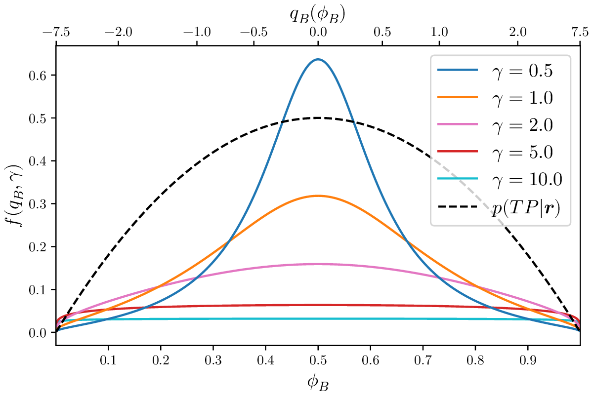
Fig. 1 Effective shooting point selection function in the committor \(\phi_B(q_B)={1}/{\left(1 + \exp(-q_B)\right)}\) through the Lorentzian selection function \(f\left(q_B, \gamma\right)\) for different values of the scale parameter \(\gamma\). \(\phi_B\) is plotted on a linear scale along the lower abscissa, the corresponding values of \(q_B(\phi_B) = - \ln \left(1 - {1}/{\phi_B}\right)\) are plotted on the upper abscissa. The reactive probability \(p(\mathrm{TP} | \symbf{r})=2 (1-\phi_B) \phi_B\) is also shown for reference. Note that, even with the default choice of \(\gamma=1\) only approximately half the probability mass is concentrated in the region \(0.3 < \phi_B < 0.7\) and from \(\gamma \approx 3\) on an almost uniform distribution along \(\phi_B\) is achieved.

Density adaption

Density adaption is the process of flattening the density of potential shooting configurations along the predicted committor to simplify the definition of a selection distribution along the committor.

Density adaption is mostly relevant in the context of RCModel-assisted shooting point selection using RCModelSPSelector (subclasses). Various density adaption schemes and many parameters are supported and specified trough the dataclass DensityAdaptionParameters.

The density adaption corrects for the fact that simply giving all potential shooting point (SP) configurations a weight equal to the Lorentz distribution with scale parameter \(\gamma\) along \(q_B(\symbf{r} | \symbf{w})\),

\[ \begin{align} f\left(q_B(\symbf{r} | \symbf{w}), \gamma\right) &= \frac{1}{\pi} \frac{\gamma}{q_B(\symbf{r} | \symbf{w})^2 + \gamma^2} , \end{align} \]

is not enough to have the SP configurations follow a Lorentz distribution in \(q_B(\symbf{r} | \symbf{w})\). The reason is that the configurations are not necessarily distributed uniformly along the committor - especially for asymmetric and/or steep barriers the density of configurations on TPs projected along \(\phi_B(\symbf{r})\) and/or \(q_B(\symbf{r} | \symbf{w})\) can be very uneven (see Fig. 2) - and the resulting selection probability \(\symbf{r}\sim p\left(\phi_B\left(q_B(\symbf{r} | \symbf{w})\right) | \mathrm{TP}\right) \, f(q_B(\symbf{r} | \symbf{w}), \gamma)\) is heavily skewed and/or shifted towards the regions where \(p\left(\phi_B\left(q_B(\symbf{r} | \symbf{w})\right) | \mathrm{TP} \right) \equiv p\left(\phi_B(\symbf{r} | \symbf{w}) | \mathrm{TP} \right)\) is high. Density adaption corrects for the imbalance by using an additional multiplicative weight proportional to the inverse of observed distribution of committor values in the potential shooting points, \(\rho_{SP}\left(\phi_B(\symbf{r} | \symbf{w})\right)\). The weight function used to select SP configurations with density adaption is therefore

\[ \begin{align} f_{sel}\left(q_B(\symbf{r} | \symbf{w})\right) = \frac{f\left(q_B(\symbf{r} | \symbf{w}), \gamma\right)}{\rho_{SP}\left(\phi_B(\symbf{r} | \symbf{w})\right)}, \end{align} \]

where the factor \(\rho_{SP}\left(\phi_B(\symbf{r} | \symbf{w})\right)\) can be estimated during the transition path sampling simulation by a histogram of \(\phi_B(\symbf{r} | \symbf{w})\) values for potential shooting configurations. Currently, two density adaption schemes are implemented in aimmd.distributed for classic TPS (in which the SP is selected from the previous accepted transition), one is correcting for the density observed along all accepted TPs, option “p_x_tp”, and the other is correcting for the density observed only on the input transition, option “lazzeri” (introduced in Lazzeri et. al. (JCTC 2023)). For TPS with a reservoir of equilibrium shooting points the only currently implemented scheme is to flatten the committor distribution observed in the shooting point reservoir. See also the docstring of DensityAdaptionParameters.

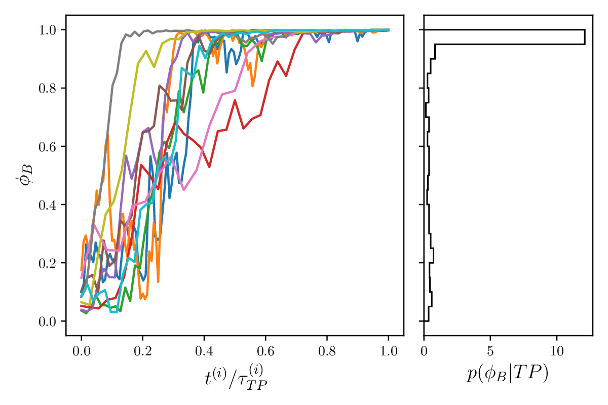
Fig. 2 Illustration of the imbalance of potential shooting point configurations projected onto \(\phi_B\). The left panel shows ten transition paths (TPs) evolving over time along \(\phi_B\) (all times are scaled to \([0,1]\) by dividing with the length of the individual transition \(\tau_{\mathrm{TP}}^{(i)}\)). The right panel shows the histogram of \(\phi_B\) values encountered on the ten TPs, i.e. an estimate for \(p(\phi_B | \mathrm{TP})\). The TPs are taken from a flexible length transition path sampling simulation between the bound (\(A\)) and unbound (\(B\)) states of \(\mathrm{Li}^{+}\mathrm{Cl}^{-}\) in water.