Symbolic Regression#
This notebook shows how to extract a low dimensional mathematical expression that approximates the committors the RCModel learned in the iterative sampling phase.
We will:
Load the previous simulation data from the
openpathsamplingstorage and load the most recentRCModelassociated with that simulationDo a HIPR analysis to identify the most relevant coordinates as found by the
RCModelUse the few most important coordinates as only inputs to the symbolic regression
Note however, that the symbolic regression is not strictly speaken a fit of the RCModel, but instead we use the same maximum likeliehood loss function as the RCModels to find the most likely reaction coordinate in the reduced space in which the symbolic regression lives. The result is therefore independant of the previously used RCModel and we do not introduce any biases through possible overfitting/underfitting in the sampling phase.
%matplotlib inline
import os
import aimmd
import numpy as np
import matplotlib.pyplot as plt
import openpathsampling as paths
import openpathsampling.engines.toy as toys
from functools import reduce
Tensorflow/Keras not available
# load a helper class for visualization of the toy system
%run resources/toy_plot_helpers.py
# change to the folder in which we previously sampled
wdir = '/home/think/scratch/SimData_pytorch_toy_22dim/'
notebook_dir = os.path.abspath(os.getcwd())
if wdir is not None:
    os.chdir(wdir)
1. Load what we need from the simulation#
trainset (to be able to calculate the HIPR and to train the symbolic regression on)
RCModel(for HIPR analysis only)toy PES for plotting
storage_file = 'pytorch_toy_22dim.nc'
storage = paths.Storage(storage_file, 'r')
toy_eng = storage.engines[0]
stateA = storage.volumes.find('StateA')
stateB = storage.volumes.find('StateB')
pes_list = []
# get the part of the potential that lies in x/y plane for plotting
ow = toy_eng.topology.pes.pes1.pes1.pes1
print('OuterWalls: ', ow)
pes_list.append(ow)

gauss1 = toy_eng.topology.pes.pes1.pes1.pes2
print('gaussian 1: ', gauss1)
pes_list.append(gauss1)

gauss2 = toy_eng.topology.pes.pes1.pes2
print('gaussian 2: ', gauss2)
pes_list.append(gauss2)

# define the energy function for plotting using the previously retrieved parameters
# i.e. the free energy of the system in x/y
def OuterWalls(x):
    return np.sum(pes_list[0].sigma[:2] * (x - pes_list[0].x0[:2])**6, axis=-1)

def GaussA(x):
    return pes_list[1].A * np.exp(np.sum(- pes_list[1].alpha[:2] * (x - pes_list[1].x0[:2])**2, axis=-1))

def GaussB(x):
    return pes_list[2].A * np.exp(np.sum(- pes_list[2].alpha[:2] * (x - pes_list[2].x0[:2])**2, axis=-1))

def V(x):
    return OuterWalls(x) + GaussA(x) + GaussB(x)
OuterWalls:  OuterWalls([0.2 1.  0.  0.  0.  0.  0.  0.  0.  0.  0.  0.  0.  0.  0.  0.  0.  0.
 0.  0.  0.  0. ], [0. 0. 0. 0. 0. 0. 0. 0. 0. 0. 0. 0. 0. 0. 0. 0. 0. 0. 0. 0. 0. 0.])
gaussian 1:  Gaussian(-0.7000000000000001, [12. 12.  0.  0.  0.  0.  0.  0.  0.  0.  0.  0.  0.  0.  0.  0.  0.  0.
  0.  0.  0.  0.], [-0.75 -0.5   0.    0.    0.    0.    0.    0.    0.    0.    0.    0.
  0.    0.    0.    0.    0.    0.    0.    0.    0.    0.  ])
gaussian 2:  Gaussian(-0.7000000000000001, [12. 12.  0.  0.  0.  0.  0.  0.  0.  0.  0.  0.  0.  0.  0.  0.  0.  0.
  0.  0.  0.  0.], [0.75 0.5  0.   0.   0.   0.   0.   0.   0.   0.   0.   0.   0.   0.
 0.   0.   0.   0.   0.   0.   0.   0.  ])
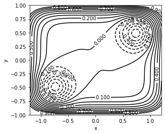
Plot the toy system energy surface in 2d#
x = np.linspace(-1.2, 1.2, 240)
y = np.linspace(-1., 1., 200)
X, Y = np.meshgrid(x,y)

coord = np.array([[xv, yv] for yv in y for xv in x])
V_val = V(coord)
V_val = V_val.reshape((len(y), len(x)))

fig, axs = plt.subplots(1)
#mapp = axs.imshow(V_val, extent=[x[0], x[-1], y[0], y[-1]], origin='lower')
axs.set_xlabel('x')
axs.set_ylabel('y')
#fig.colorbar(mapp)

levels = np.arange(-1.5 , 1., 0.1)
CS = axs.contour(X, Y, V_val, levels, colors='k')
axs.clabel(CS, inline=1, fontsize=10, )
axs.set_aspect('equal')
open aimmd storage#
aimmd_storage = aimmd.Storage("aimmd_storage.h5", "r")
Load the trainingset#
trainset = aimmd_storage.load_trainset()
Load the model#
model = aimmd_storage.rcmodels["most_recent"]
model = model.complete_from_ops_storage(storage)
aimmd storage passed as density collector cache file is open in read-only mode. No appending will be possible.
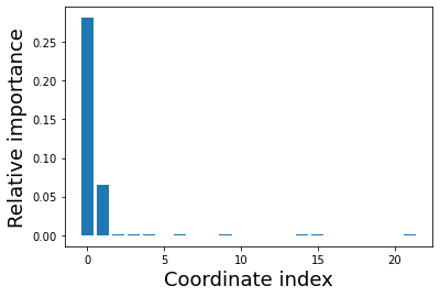
2. Do a HIPR analysis to find the most relevant input coordinates#
hipr = aimmd.analysis.HIPRanalysis(model, trainset)
hipr_plus_losses, hipr_plus_std = hipr.do_hipr_plus()
# plot the loss differences
fig, axs = plt.subplots(1)
plt.bar(np.arange(len(hipr_plus_losses)-1), hipr_plus_losses[:-1] - hipr_plus_losses[-1])
plt.xlabel('Coordinate index', size=18)
plt.ylabel('Relative importance', size=18);
# Note that this is a bit pointless for the toy system, as we know that only the first two are relevant
# But it is nice to see that the RCmodel thinks so too :)
3. Symbolic regression#
# necessary imports
import pyaudi
import sympy as sp
# find the most relevant coordinates, i.e. where loss difference is maximal
loss_plus_diffs = hipr_plus_losses[:-1] - hipr_plus_losses[-1]
max_idxs = np.argsort(loss_plus_diffs)[::-1]
print('Most relevant coordinate indices: ', max_idxs)
print('Should have 0, 1 as first two entries for the toy system.')
# get the descriptors and shot results as numpy arrays from the training set
descriptors = trainset.descriptors
shot_results = trainset.shot_results
Most relevant coordinate indices:  [ 0  1 14 15  4  3  2  6 21  9 19 12  7 16 10 17  5 11 20 18 13  8]
Should have 0, 1 as first two entries for the toy system.
n = 2  # lets take the two most relevant inputs for the symbolic regression,
       # i.e. our resulting low dimensional reaction coordinate expression will be of dimension 2
skip = 2  # take only every Nth step to speed up stuff a bit, [should not change the result drastically as subsequent shooting points are correlated anyways]

# create training inputs for symbolic regression
# the training inputs need to be gdual_vdoubles, since we need to be able to calculate gradients w.r.t. them
xt = [pyaudi.gdual_vdouble(descriptors[::skip, i]) for i in max_idxs[:n]]
# the targets can (and should for efficiency) also be numpy arrays, since we need no gradients for them
yt = shot_results[::skip]

# take all points for calculating the test loss
xtf = [pyaudi.gdual_vdouble(descriptors[:, i]) for i in max_idxs[:n]]
ytf = shot_results[:]
# initialize symbolic regression expression with random conectivity and random edge weights
expression = aimmd.symreg.initialize_random_expression(n,  # n inputs
                                                      1,  # 1 output: p_B
                                                      kernels=['sum', 'diff', 'mul', 'div', 'log', 'exp'], # potentially allowed elementary mathematical operations
                                                                                                           # our final expression will be a combination of those operations
                                                                                                           # could also add 'sin' and 'sig' for sine and sigmoid
                                                     )
# choose a loss function and a complexity regularization
lossFX = aimmd.symreg.losses.binom_loss  # binmial loss for models predicting p_B in a two state system
complex_fx = lambda ex: aimmd.symreg.losses.operation_count(ex, fact=0.0001)  # operation_count counts the number of elementary mathematical operations in the expression
complex_fx_reduced = lambda ex: aimmd.symreg.losses.operation_count(ex, fact=0.00001)  # and multiplies it with factor to get a loss contribution

# there are also other complexity penalties available
# aimmd.symreg.losses.active_genes_count : penalizes number of actives genes in the expression
# aimmd.symreg.losses.l1_regularization : sparsity regularization on the edge weights
# aimmd.symreg.losses.l2_regularization : penalize length of the vector of edge weights (not really a complexity penalty, but sometimes useful)
# here we optimize the expression
lossL = []
genesL = []
weightsL = []
n_iter = 4  # do it n_iter times in a row to get a feeling for the stability of the result
for _ in range(n_iter):
    # initilize a new random expression every time, otherwise we would start the genetic algorithm from the previously optimized individual
    # (which would be the same as running one optimization n_iter times longer)
    expression = aimmd.symreg.initialize_random_expression(n, 1, kernels=['sum', 'diff', 'mul', 'div', 'log', 'exp'])
    loss, genes, weights = aimmd.symreg.optimize_expression(expression, # expression to optimize
                                                           4,  # number of mutants to create in every generation
                                                           100, # maximum number of generations
                                                           xt,  # training points
                                                           yt,  # training targets, i.e. shot results
                                                           lossFX,  # either binomial loss for 2 state (predicting only p_B) or multinomial loss for N state
                                                           complexity_regularization=complex_fx,  # the combined lambda function(s) we use for complexity regularization
                                                                                                  # all of these do not need gradients w.r.t the weights
                                                           weight_regularization=None,  # combined lambda functions for weight regularizations
                                                                                        # these need and calculate the gradients w.r.t. edge weights
                                                           newtonParams={'steps':100},  # newton steps is what makes up most of the runtime,
                                                                                        # however if it is to small expressions will not converge in parameter space
                                                                                        # this can be diagnosed if we have many similar expression with different coeffs
                                                          )
    # store loss, genes and weights of the best expression found in every round
    lossL.append(loss)
    genesL.append(genes)
    weightsL.append(weights)
/home/think/.conda/envs/aimmd_nature_publish/lib/python3.8/site-packages/numpy/linalg/linalg.py:2158: RuntimeWarning: invalid value encountered in det
  r = _umath_linalg.det(a, signature=signature)
losses_sans_regul = []
# print the resulting equations for every round
for l, g, w in zip(lossL, genesL, weightsL):
    # we take a dummy expression and set it to the optimal parameters we found previously
    expression.set(g)  # set genes to the best we found
    expression.set_weights(w)  # also set edge weights of the expression
    print('loss with regularization on training data: ', l)  # this is the loss we had in training, includes all regularizations and is calculated only over the reduced dataset
    print('losss without regularization on all data: ', sum(lossFX(expression, xtf, ytf).constant_cf))  # this is the loss of the expression on the full dataset without regularizations
                                                                                                        # i.e. the actual likeliehood
    losses_sans_regul += [sum(lossFX(expression, xtf, ytf).constant_cf)]
    print(expression.simplify(['x{:d}'.format(idx) for idx in max_idxs[:n]], subs_weights=True))  # print the formula, subsitute edge weights to numbers
    print()
loss with regularization on training data:  0.5511955319233025
losss without regularization on all data:  0.557085855753694
[0.388417665364765*x0**2 + 3.14832759089886*x0 + 1.54435987411918*x1]

loss with regularization on training data:  0.551387755402174
losss without regularization on all data:  0.5577538719638445
[3.14141874229458*x0 + 1.53836637022338*x1]

loss with regularization on training data:  0.5470211251747448
losss without regularization on all data:  0.5504382796275298
[x0*(3.28883990138331 - 3.55898427657923*x1) + x1**2*(0.0742680371108349*x0 + 0.00287435906260654*x1 + 0.0201049408547817)/(0.73195646062766*x0 + 0.0283285484292352*x1) + x1*((0.929750658205071*x0 + 0.0359836793099553*x1)*exp(2.22632568182177*x0) + 0.00297151954213768)/(0.73195646062766*x0 + 0.0283285484292352*x1)]

loss with regularization on training data:  0.5453408962587112
losss without regularization on all data:  0.5470560701405641
[5.83027324700111*x0**2*x1 + x0*(4.31828543011026*x1**2 + 2.95933640738348) + 1.26018191728888*x1]
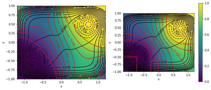
Plot the committor predicted by the symbolic regression expression onto the potential#
Also load and plot the exact committor for the 2D energy surface, the method for the calculation can be found in “Molecular free energy profiles from force spectroscopy experiments by inversion of observed committors” (Covino, Woodside, Hummer, Szabo and Cossio; J. Chem. Phys. 151, 154115 (2019); https://doi.org/10.1063/1.5118362).
# Note that since the symbolic regression predicts log_probabilities we will need to take the sigmoid to get p_B
# we use scipy for that
from scipy.special import expit as sigmoid
# choose an expression to plot and get the weights + genes we stored
expr_idx = np.argmin(losses_sans_regul)
print(f"Chose expression with index {expr_idx} for plotting, because it has the lowest loss.")
genes = genesL[expr_idx]
weights = weightsL[expr_idx]
# set genes and weights as above
expression.set(genes)
expression.set_weights(weights)

# genereate the energy surface plotting data
x = np.linspace(-1.2, 1.2, 240)
y = np.linspace(-1., 1., 200)
X, Y = np.meshgrid(x,y)
# create an array of coordinate value pairs to calculate V(x,y)
# do it as one big 1d array as it is much faster
coord = np.array([[xv, yv] for yv in y for xv in x])
V_val = V(coord)
# unwrap to a 2d array for plotting
V_val = V_val.reshape((len(y), len(x)))

# generate RC plotting data
coord_gdual = [pyaudi.gdual_vdouble(coord[:, i]) for i in range(coord.shape[1])]
rc = expression(coord_gdual)  # this is now a list of gdual_vdoubles
# since we trained with the binomial loss the RC only has one entry, the RC towards B
rc = np.array(rc[0].constant_cf) # convert to a numpy array, i.e. take only the values and ignore the higher order derivates
# again unwrap to 2d array for plotting
rc_mat = rc.reshape((len(y), len(x)))
symreg_committor = sigmoid(rc_mat)

# load exact committor
exact_commitor = np.load(os.path.join(notebook_dir, "resources", "toy_exact_committor.npy")).T

# actual plotting
fig, axs = plt.subplots(ncols=2, figsize=(12, 5))
for axnum, (data, title, ax) in enumerate(zip([symreg_committor, exact_commitor],
                                              ["Symbolic regression", "Exact committor"],
                                               axs)):
    ax.set_xlabel('x')
    ax.set_ylabel('y')

    # plot isolines of the energy surface
    levels = np.arange(-1.5 , 1., 0.1)
    CS = ax.contour(X, Y, V_val, levels, colors='k')
    ax.clabel(CS, inline=1, fontsize=10, )
    #ax.set_aspect('equal')


    # first as color gradient
    mapp = ax.imshow(data, extent=[x[0], x[-1], y[0], y[-1]], origin='lower')
    # also plot isolines of p_B in red
    levels = np.arange(0. , 1., 0.1)
    CS = ax.contour(X, Y, data, levels, colors='r')
    ax.clabel(CS, inline=1, fontsize=10, )

# draw a colorbar
fig.colorbar(mapp)
Chose expression with index 3 for plotting, because it has the lowest loss.
<matplotlib.colorbar.Colorbar at 0x7f81a5676c70>