Massively parallel Transition Path Sampling#
Notebook 3: Analyze TPS simulation#
This is the third of a series of example notebooks on massively parallel transition path sampling. Obviously you need to have run the TPS simulation in the first notebook to analyze it here (you do not necesarily have to continue it in the second notebook).
We will first have a look at the training of the model during the simulation and also at its ability to predict the shooting outcomes accurately (using the difference between expected and actual outcomes). We will perform a relative input importance analysis to see which input descriptors influence the reaction coordinate models prediction the most (these are the important coordinates determining the committor and describing the reaction). Finaly we will project the density of transitions to the \(\psi\),\(\phi\) plane and (hopefully) observe that all the Markov chains converged to the same density.
This notebook should be run on a multi-core workstation preferably with a GPU, otherwise you will have a very long coffee break and a very hot laptop.
Required knowledge/recommended reading: This notebooks assumes some familarity with the asyncmd (namely the [gromacs] engine and TrajectoryFunctionWrapper classes). Please see the example notebooks in asyncmd for an introduction.
Imports and set working directory#
%matplotlib inline
import os
import asyncio
import numpy as np
import matplotlib.pyplot as plt
import mdtraj as mdt
import MDAnalysis as mda
import aimmd
import aimmd.distributed as aimmdd
import asyncmd
import asyncmd.trajectory as asynctraj
from asyncmd import Trajectory
/home/think/.conda/envs/aimmd_dev/lib/python3.10/site-packages/tqdm/auto.py:22: TqdmWarning: IProgress not found. Please update jupyter and ipywidgets. See https://ipywidgets.readthedocs.io/en/stable/user_install.html
  from .autonotebook import tqdm as notebook_tqdm
Could not initialize SLURM cluster handling. If you are sure SLURM (sinfo/sacct/etc) is available try calling `asyncmd.config.set_slurm_settings()` with the appropriate arguments.
Tensorflow/Keras not available
# setup working directory (this should be the same as in the previous notebook)
scratch_dir = "."

workdir = os.path.join(scratch_dir, "TransitionPathSampling_ala")
Open the storage in read only mode#
storage = aimmd.Storage(os.path.join(workdir, "storage.h5"), mode="r")
Opening storage without write intent, asyncmd trajectory value caching will not be performed in h5py (but most likely as seperate npz files).
Load the model, trainset and brain#
We do not realy need them but it can be most comfortable to access the simulation results via the brain (e.g. the order of accepted MC steps globaly).
model = storage.rcmodels["model_to_continue_with"]
aimmd storage passed as density collector cache file is open in read-only mode. No appending will be possible.
trainset = storage.load_trainset()
tasks = [aimmdd.pathsampling.TrainingTask(model=model, trainset=trainset),
         aimmdd.pathsampling.SaveTask(storage=storage, model=model, trainset=trainset),
         aimmdd.pathsampling.DensityCollectionTask(model=model,
                                                   first_collection=100,
                                                   recreate_interval=500,
                                                   ),
         ]
brain = storage.load_brain(model=model, tasks=tasks)
brain.total_steps
10018
Plot the training of the model during the simulation#
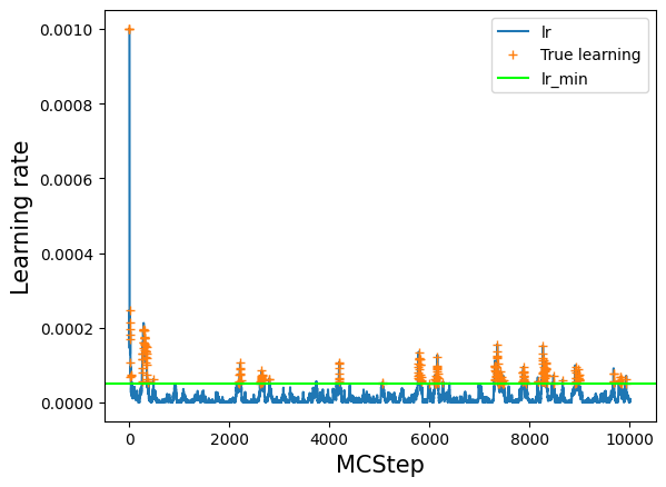
Learning rate vs Monte Carlo step#
# lets have a look at the value of the learning rate over the course of training
# note however, that we did not train at every step, but just at every interval MCsteps
log_train = np.array(model.log_train_decision)
lr = log_train[:,1]
plt.plot(lr, label='lr')
# see where we really trained: everywhere where train=True
# set lr_true to NaN anywhere where we did not train to have a nice plot
lr_true = lr
lr_true[log_train[:,0] == False] = np.nan
plt.plot(lr_true, '+', label='True learning')
# lr_min as a guide to the eye
plt.axhline(model.ee_params['lr_min'], label='lr_min', color='lime')
plt.legend()
plt.xlabel('MCStep', size=15);
plt.ylabel('Learning rate', size=15);
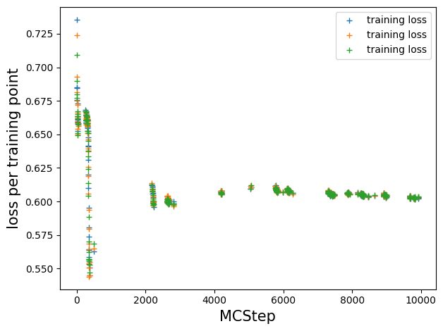
Loss vs Monte Carlo step#
# resort such that we have a loss value per MCStep, NaN if we did not train at that step
train_loss = []
count = 0
for t in log_train[:, 0]:
    if t:
        train_loss.append(model.log_train_loss[count])
        count += 1
    else:
        train_loss.append([np.nan for _ in range(model.ee_params['epochs_per_train'])])

plt.plot(train_loss, '+', label='training loss')
plt.legend();
plt.ylabel('loss per training point', size=15)
plt.xlabel('MCStep', size=15)
plt.tight_layout()
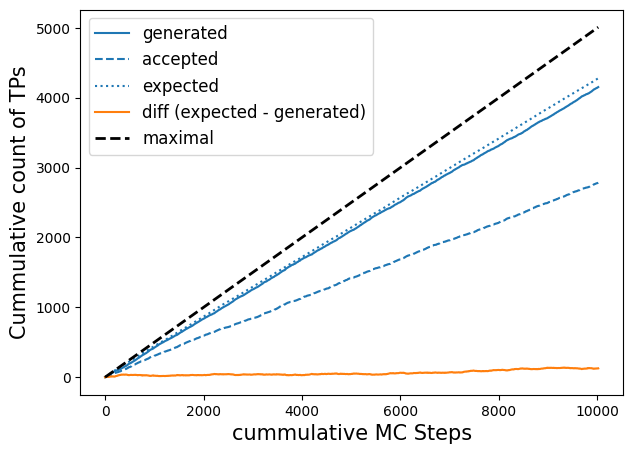
Cumulative counts of expected, generated and accepted transitions vs Monte Carlo step#
# plot efficiency, expected efficiency and accepts
# Note: this will only work for models with n_out=1, due to the way we calculate p(TP|x)
fig, axs = plt.subplots(figsize=(7, 5))

n_steps = -1  # up to which step number to plot

p_ex = np.array(model.expected_p)[:n_steps]

l, = axs.plot(np.cumsum(trainset.transitions[:n_steps]), label='generated');
axs.plot(np.cumsum(brain.accepts[:n_steps]), c=l.get_color(), ls='--', label='accepted');
axs.plot(np.cumsum(2*p_ex*(1 - p_ex)),c=l.get_color(), ls=':', label='expected');
axs.plot(np.cumsum(2*p_ex*(1 - p_ex))- np.cumsum(trainset.transitions[:n_steps]), label='diff (expected - generated)')
axs.plot(np.linspace(0., len(trainset[:n_steps])/2., len(trainset[:n_steps])), c='k', ls='--', label='maximal', lw=2)
axs.legend(fontsize=12);
axs.set_ylabel('Cummulative count of TPs', size=15)
axs.set_xlabel('cummulative MC Steps', size=15);
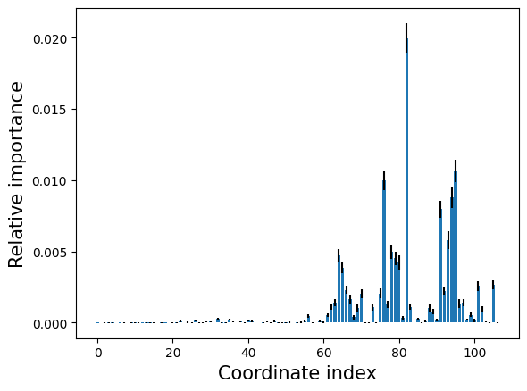
Relative input importance analysis#
We will use the hipr class to perform the input importance analysis, it randomizes each coordinate one at a time and calculates the resulting losses.
hipr = aimmd.analysis.HIPRanalysis(model, trainset)
# do 100 repetitions, return mean and std
hipr_plus_losses, hipr_plus_stds = hipr.do_hipr_plus(100)
Plot the loss increase (relative importance) of each coordinate#
loss_diffs = hipr_plus_losses[:-1] - hipr_plus_losses[-1]  # hipr_losses[-1] is the reference loss over the unaltered trainset

plt.bar(np.arange(len(loss_diffs)), loss_diffs, yerr=hipr_plus_stds[:-1])
plt.xlabel('Coordinate index', size=15)
plt.ylabel('Relative importance', size=15);
Print out the most important coordinates#
We try our best to print out the most relevant coordinates in a human understandeable form.
# what are the most important contributors?
max_idxs = np.argsort(loss_diffs)[::-1]

# import the function used to generate the internal coordinate representation for the molecule
from state_funcs_mda import generate_atomgroups_for_ic

# and use it to get lists of pairs (distances), triples (angles) and quadruples ([pseudo-]dihedrals)
u = mda.Universe("gmx_infiles/ala_300K_amber99sb-ildn.tpr", "gmx_infiles/conf.gro",
                 refresh_offsets=True, tpr_resid_from_one=True)
molecule = u.select_atoms('protein')
pairs, triples, quadruples = generate_atomgroups_for_ic(molecule)

def pprint_atom(at):
    """Helper function to print atom information in a nice way."""
    ret = f"Atom {at.ix+1}:"
    if hasattr(at, "name"):
        ret += f" {at.name}"
    if hasattr(at, "resname"):
        ret += f" in residue {at.resname}"
    if hasattr(at, "resid"):
        ret += f" (resid {at.resid})"
    return ret

# now use all of this to print the most relevant coordinates in a remotely human understandable fashion
print('reference loss:', hipr_plus_losses[-1])
for idx in max_idxs[:7]:
    print()
    print('loss for idx {:d}: '.format(idx), hipr_plus_losses[idx], f" (loss diff= {hipr_plus_losses[idx] - hipr_plus_losses[-1]})")
    if idx < len(pairs[0]):
        print(f"bond between: {pprint_atom(pairs[0][idx])} and {pprint_atom(pairs[1][idx])}")
        continue
    idx -= len(pairs[0])
    if idx < len(triples[0]):
        print(f"angle between {pprint_atom(triples[0][idx])}, {pprint_atom(triples[1][idx])} and {pprint_atom(triples[2][idx])}")
        continue
    idx -= len(triples[0])
    if idx % 2 == 0:
        st = "sinus"
    else:
        st = "cosinus"
    st += f" of dihedral between {pprint_atom(quadruples[0][idx // 2])}, {pprint_atom(quadruples[1][idx // 2])}, {pprint_atom(quadruples[2][idx // 2])}"
    st += f" and {pprint_atom(quadruples[3][idx // 2])}."
    print(st)
reference loss: 0.600353531124445

loss for idx 82:  0.6203346194866817  (loss diff= 0.019981088362236665)
cosinus of dihedral between Atom 7: N in residue ALA (resid 2), Atom 9: CA in residue ALA (resid 2), Atom 15: C in residue ALA (resid 2) and Atom 17: N in residue NME (resid 3).

loss for idx 95:  0.6109904614321175  (loss diff= 0.010636930307672543)
sinus of dihedral between Atom 11: CB in residue ALA (resid 2), Atom 9: CA in residue ALA (resid 2), Atom 15: C in residue ALA (resid 2) and Atom 17: N in residue NME (resid 3).

loss for idx 76:  0.6103401733325327  (loss diff= 0.009986642208087648)
cosinus of dihedral between Atom 7: N in residue ALA (resid 2), Atom 9: CA in residue ALA (resid 2), Atom 11: CB in residue ALA (resid 2) and Atom 12: HB1 in residue ALA (resid 2).

loss for idx 94:  0.6091335810385057  (loss diff= 0.008780049914060672)
cosinus of dihedral between Atom 10: HA in residue ALA (resid 2), Atom 9: CA in residue ALA (resid 2), Atom 15: C in residue ALA (resid 2) and Atom 16: O in residue ALA (resid 2).

loss for idx 91:  0.6083131660618308  (loss diff= 0.007959634937385829)
sinus of dihedral between Atom 10: HA in residue ALA (resid 2), Atom 9: CA in residue ALA (resid 2), Atom 11: CB in residue ALA (resid 2) and Atom 14: HB3 in residue ALA (resid 2).

loss for idx 93:  0.6061324184339284  (loss diff= 0.005778887309483394)
sinus of dihedral between Atom 10: HA in residue ALA (resid 2), Atom 9: CA in residue ALA (resid 2), Atom 15: C in residue ALA (resid 2) and Atom 16: O in residue ALA (resid 2).

loss for idx 78:  0.6053583165780112  (loss diff= 0.005004785453566196)
cosinus of dihedral between Atom 7: N in residue ALA (resid 2), Atom 9: CA in residue ALA (resid 2), Atom 11: CB in residue ALA (resid 2) and Atom 13: HB2 in residue ALA (resid 2).
Analyze the transition path ensemble#
We will have a look at the density of transitions and shootin points in the \(\psi\), \(\phi\) plane and at the transition time distribution. Note that instead of a function projecting the trajectories to the \(\psi\), \(\phi\) plane, you could use any function that projects configurations to lower dimensional spaces or calculates scalars over whole trajectories (as for the distribution of transition times).
# import a function to project the trajectory data to the ψ, φ plane
from state_funcs_mda import descriptor_func_psi_phi
# wrapp it to make it awaitable
wrapped_psi_phi = asynctraj.PyTrajectoryFunctionWrapper(descriptor_func_psi_phi)
# get out all mcstates (sorted by collection so we can compare the collections to each other later below)
# Note that the mcstates contains doubles because the represent the chain of acceppted Monte Carlo steps (in case of a reject we reaccept)
mcstates_by_collection = [[state for state in collection.mcstates()] for collection in storage.mcstep_collections]
# calculate all ψ,φ values for all transitions for plotting later
accepted_steps_psi_phi_by_collection = []
for collection_states in mcstates_by_collection:
    accepted_steps_psi_phi_by_collection.append(await asyncio.gather(*(wrapped_psi_phi(s.path) for s in collection_states)))
# get all SPs (and all accepted ones separately) out of the storage
SPs_accepted = [[] for _ in range(len(storage.mcstep_collections))]
SPs_success = [[] for _ in range(len(storage.mcstep_collections))]
SPs_all = [[] for _ in range(len(storage.mcstep_collections))]

for cidx, step_collection in enumerate(storage.mcstep_collections):
    # we exclude the zeroth step as it has now shoting_snap (it is our initial transition)
    for step in step_collection[1:]:
        SPs_all[cidx] += [step.shooting_snap]
        if step.path is not None:
            # we generated a transition
            SPs_success[cidx] += [step.shooting_snap]
        if step.accepted:
            # and accepted it
            SPs_accepted[cidx] += [step.shooting_snap]
# calculate ψ and φ values for all SPs for plotting later
sps_all_psi_phi = []
sps_success_psi_phi = []
sps_accepted_psi_phi = []

for cidx in range(len(SPs_all)):
    sps_all_psi_phi += [await asyncio.gather(*(wrapped_psi_phi(sp) for sp in SPs_all[cidx]))]
    sps_success_psi_phi += [await asyncio.gather(*(wrapped_psi_phi(sp) for sp in SPs_success[cidx]))]
    sps_accepted_psi_phi += [await asyncio.gather(*(wrapped_psi_phi(sp) for sp in SPs_accepted[cidx]))]
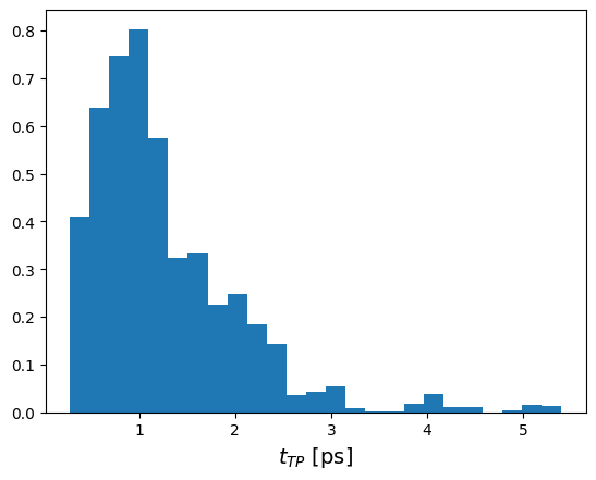
Plot the transition path time distribution#
# get out the number of frames for each transition
t_TP_in_frames = [len(s.path) for s in collection_states for collection_states in mcstates_by_collection]

# get our MDP file so we can find out how long the timedifference between frames is
# (all our samplers are the same and have only one mover each)
mdp = brain.samplers[0].movers[0].engine_kwargs["mdconfig"]
# we write XTC trajectories so this is the relevant output frequency
timediff_per_frame_in_ps = mdp["dt"] * mdp["nstxout-compressed"]
# and plot transition path time distribution
fig, axs = plt.subplots()

axs.hist(np.array(t_TP_in_frames) * timediff_per_frame_in_ps,
         bins=25, density=True)
axs.set_xlabel("$t_{TP}$ [ps]", size=14);
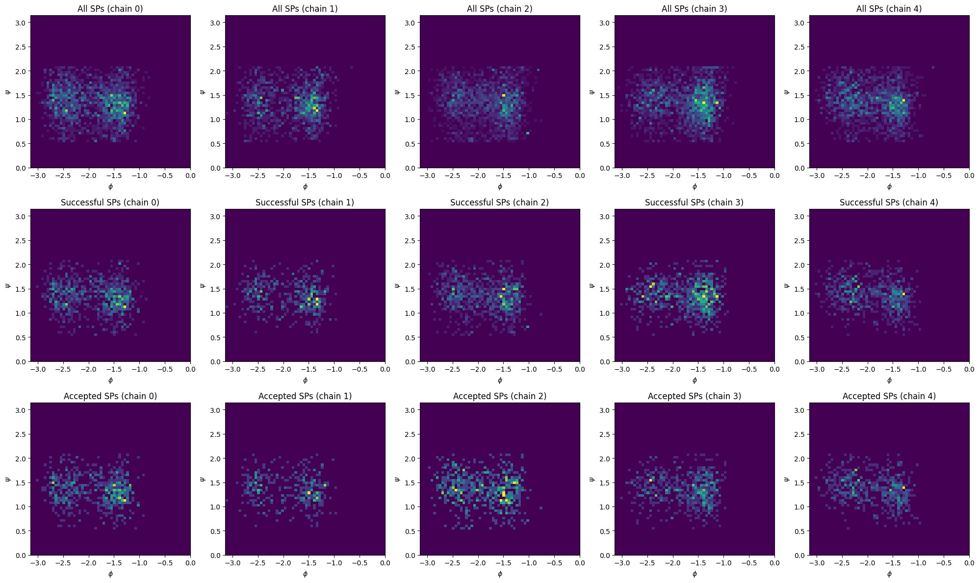
Plot the density of shooting points (SPs) in the \(\psi\), \(\phi\) plane#
fig, axs = plt.subplots(ncols=len(storage.mcstep_collections), nrows=3,
                        figsize=(len(storage.mcstep_collections)*4, 12))

for dataidx, (data, axs_array) in enumerate(zip([sps_all_psi_phi, sps_success_psi_phi, sps_accepted_psi_phi], axs)):
    for cidx, ax in enumerate(axs_array):
        if dataidx == 0:
            title = "All SPs"
        elif dataidx == 1:
            title = "Successful SPs"
        elif dataidx == 2:
            title = "Accepted SPs"
        title += f" (chain {cidx})"
        ax.set_title(title)
        ax.set_xlabel("$\phi$")
        ax.set_ylabel("$\psi$")
        plot_data = np.concatenate(data[cidx], axis=0)
        ax.hist2d(plot_data[:, 1], plot_data[:, 0], bins=(60, 60), range=((-np.pi, 0), (0, np.pi)), density=True)
        ax.set_xlim(-np.pi, 0)
        ax.set_ylim(0, np.pi)

fig.tight_layout()
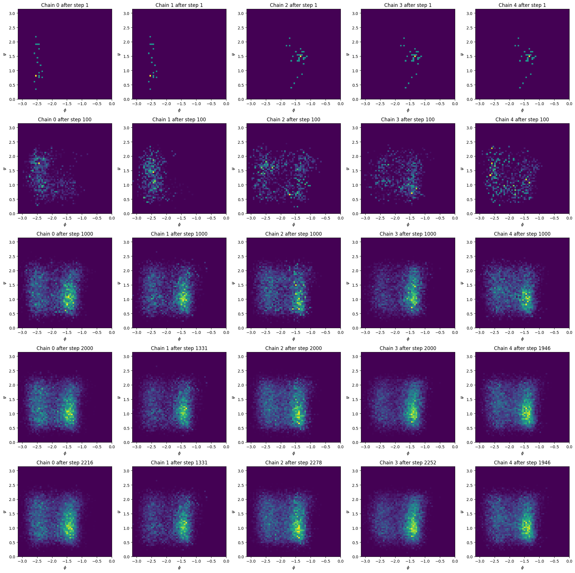
Plot the density of transitions in the \(\psi\), \(\phi\) plane, \(p(\psi,\phi|TP)\)#
steps_done = [1, 100, 1000, 2000, None]  # the None gives us the last step for all chains

fig, axs = plt.subplots(ncols=len(storage.mcstep_collections), nrows=len(steps_done),
                        figsize=(len(storage.mcstep_collections)*4, 4*len(steps_done)))

for max_step, axs_array in zip(steps_done, axs):
    for c_idx, ax in enumerate(axs_array):
        ax.set_title(f"Chain {c_idx} after step {len(accepted_steps_psi_phi_by_collection[c_idx][:max_step])}")
        ax.set_xlabel("$\phi$")
        ax.set_ylabel("$\psi$")
        plot_data = np.concatenate(accepted_steps_psi_phi_by_collection[c_idx][:max_step], axis=0)
        ax.hist2d(plot_data[:, 1], plot_data[:, 0], bins=(60, 60), range=((-np.pi, 0), (0, np.pi)), density=True)
        ax.set_xlim(-np.pi, 0)
        ax.set_ylim(0, np.pi)

fig.tight_layout()
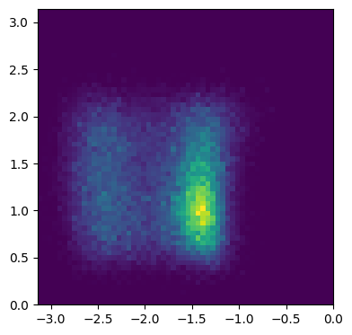
Calculate \(p(\psi,\phi|TP)\) for all chains together#
fig, axs = plt.subplots(figsize=(4, 4))

all_psi_phi = []
for i in range(len(brain.samplers)):
    all_psi_phi.append(np.concatenate(accepted_steps_psi_phi_by_collection[i], axis=0))

all_psi_phi = np.concatenate(all_psi_phi, axis=0)
combined_density, xedges, yedges = np.histogram2d(all_psi_phi[:, 1], all_psi_phi[:, 0], bins=(60, 60), range=((-np.pi, 0), (0, np.pi)), density=True)

axs.imshow(combined_density.T, extent=[xedges[0], xedges[-1], yedges[0], yedges[-1]], origin="lower")
ax.set_xlabel("$\phi$")
ax.set_ylabel("$\psi$")

fig.tight_layout()
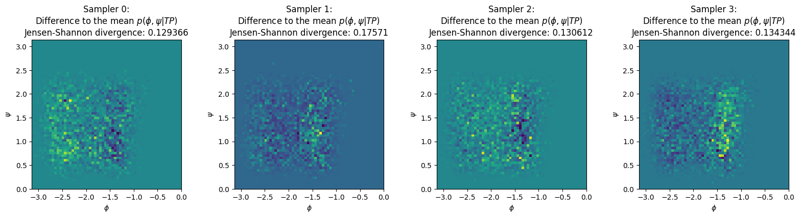
Calculate how much each Markov chain differs from the mean#
from scipy.spatial import distance
histo_per_collection = []
for i in range(len(brain.samplers)):
    plot_data = np.concatenate(accepted_steps_psi_phi_by_collection[i], axis=0)
    h, xedges, yedges = np.histogram2d(plot_data[:, 1], plot_data[:, 0], bins=(60, 60), range=((-np.pi, 0), (0, np.pi)), density=True)
    histo_per_collection.append(h)
fig, axs = plt.subplots(ncols=4, figsize=(4*4, 4))

for cidx, (h, ax) in enumerate(zip(histo_per_collection, axs)):
    q = h.T
    p = combined_density.T
    mapp = ax.imshow(q - p, extent=[xedges[0], xedges[-1], yedges[0], yedges[-1]], origin="lower")
    ax.set_title(f"Sampler {cidx}:\nDifference to the mean $p(\phi, \psi| TP)$\nJensen-Shannon divergence: {round(distance.jensenshannon(p.flatten(), q.flatten()), 6)}")
    ax.set_xlabel("$\phi$")
    ax.set_ylabel("$\psi$")

fig.tight_layout()
Find the cummulative timedifference between subsequent shooting points#
This quantity can give you an estimate on how different your shooting points are (e.g. how far a lipid could potentially diffuse from your first to your last shooting point in a chain), you should however treat it with care as we this timedifference does not necessarily equal the same timedifference in an equilibrium simulation (because we always “reset” the trajectory to be on a transition path every time we shoot).
async def SP_framediff_from_stepcollection(stepcollection, distancefunction=model.descriptor_transform):
    # this function goes through an mcstepcollection and returns the total framedifference between subsequent shooting points
    # we expect distance function to be any wrapped function returning an array of values for each frame,
    # here we will find the framediff by searching for the two SPs on the last TP in descriptor space
    # we could however use any other function (e.g. atomic positions in cartesian space) that is able to discriminate between the configurations
    idx = 0
    step = stepcollection[idx]
    last_accepted_step = None
    total_frame_diff = 0
    while idx < len(stepcollection) - 1:
        # find the first/next step that is accepted and has a shooting snap
        # (this means it was a shooting move and produced an accepted transition)
        while (idx < len(stepcollection) - 1) and ((step.shooting_snap is None) or not step.accepted):
            idx += 1
            step = stepcollection[idx]
        if last_accepted_step is None:
            last_accepted_step = step
        else:
            last_sp = last_accepted_step.shooting_snap
            this_sp = step.shooting_snap
            last_tp = last_accepted_step.path
            d_last_sp, d_this_sp, d_last_tp = await asyncio.gather(*(distancefunction(d) for d in [last_sp, this_sp, last_tp]))
            # find the frames of the SPs in tp
            frame_idx_last_sp = frame_idx_this_sp = None
            for frame_idx, frame in enumerate(d_last_tp):
                # TODO: theses tolerances are quite large but seem to be the lowest ones that work reliably?!
                if np.allclose(frame, d_last_sp, rtol=1e-2, atol=1e-2):
                    frame_idx_last_sp = frame_idx
                if np.allclose(frame, d_this_sp, rtol=1e-2, atol=1e-2):
                    frame_idx_this_sp = frame_idx
            # make sure we found them both
            assert frame_idx_last_sp is not None
            assert frame_idx_this_sp is not None
            # get the unsigned diff
            diff = abs(frame_idx_last_sp - frame_idx_this_sp)
            total_frame_diff += diff
            # and set this step to last step for further iterations
            last_accepted_step = step

        if idx < len(stepcollection) -1:
            idx += 1 # and on to the next accepted step
            step = stepcollection[idx]

    return total_frame_diff
framediffs_per_stepcollection = await asyncio.gather(*(SP_framediff_from_stepcollection(sc) for sc in storage.mcstep_collections))
timediffs_per_stepcollection = np.array(framediffs_per_stepcollection) * timediff_per_frame_in_ps
for i, td in enumerate(timediffs_per_stepcollection):
    print(f"Sampler {i} did a cummulative timedifference between SPs of {round(td, 4)} ps")
Sampler 0 did a cummulative timedifference between SPs of 215.28 ps
Sampler 1 did a cummulative timedifference between SPs of 131.36 ps
Sampler 2 did a cummulative timedifference between SPs of 212.28 ps
Sampler 3 did a cummulative timedifference between SPs of 215.68 ps
Sampler 4 did a cummulative timedifference between SPs of 178.72 ps
storage.close()