22 dimensional toy system setup with a pytorch MultiDomain RCmodel

This notebook is basically the same setup as 1_Toy_pytorch_simple_setup.ipynb but uses a MultiDomainModel. It will show you the basic usage of arcd, you will learn how to:

• set up an ANN-enhanced TPS simulation of a 22 dimensional toy system from scratch

• run the simulation

• inspect the training process

• (try to) analyze what the ANN learned

imports, working directory and logging setup

%matplotlib inline

import os
import arcd
import torch
import numpy as np
import matplotlib.pyplot as plt
import openpathsampling as paths
# convenience for the toy dynamics
import openpathsampling.engines.toy as toys
from functools import reduce

Using TensorFlow backend.

# load a helper class for visualization of the toy system
%run resources/toy_plot_helpers.py

# setup logging
# executing this file sets the variable LOGCONFIG, which is a dictionary of logging presets 
%run resources/logconf.py

# change to the working directory of choice
wdir = None
if wdir is not None:
    os.chdir(wdir)

# you can either modify single values or use it as is to get the same setupt as in the OPS default logging config file
# you could e.g. do LOGCONF['handlers']['stdf']['filename'] = new_name to change the filename of the log
# the default is to create 'simulation.log' and 'initialization.log' in the current working directory
import logging.config
logging.config.dictConfig(LOGCONFIG)

toy system setup

This is not yet arcd specific, but the general way of setting up an OPS TPS simulation, have a look at the opepathsampling example notebooks for more.

PES

• construct a 22 dimensional PES, where the first two dimensions are x and y of the plotted 2D ToyPotential, the remaining 20 dimensions are uncoupled harmonic oscillators with random frequencies to emulate irrelevant coordinates

• from a previous run in this potential we know: \(<t_{TP}>\approxeq 566 ~\mathrm{timesteps} = 11.32 ~\mathrm{units~of~time}\) => any harmonic oszilator with \(\omega < 2\pi/T \approxeq 0.555\) has a lower frequency than the transition of interest

• to challenge the ANN we make sure that the first two harmonic oscillators (i.e. dim 3 and 4) have an \(\omega\) smaller than and comparable to the transition frequency respectively

# Construct the PES as a sum of simpler PES
# Toy_PES supports adding/subtracting various PESs. 
# The OuterWalls PES type gives an x^6+y^6 boundary to the system.
n_harmonics = 20
pes_list = []
pes_list += [toys.OuterWalls(sigma=[0.2, 1.0] + [0. for _ in range(n_harmonics)],
                             x0=[0.0, 0.0] + [0. for _ in range(n_harmonics)])
            ]
pes_list += [toys.Gaussian(A=-.7,
                           alpha=[12.0, 12.0] + [0. for _ in range(n_harmonics)],
                           x0=[-.75, -.5] + [0. for _ in range(n_harmonics)])
            ]
pes_list += [toys.Gaussian(A=-.7,
                           alpha=[12.0, 12.0] + [0. for _ in range(n_harmonics)],
                           x0=[.75, .5] + [0. for _ in range(n_harmonics)])
            ]
pes_list += [toys.HarmonicOscillator(A=[0., 0.] + [1./2. for _ in range(n_harmonics)],
                                     omega=[0., 0.] + [0.2, 0.5] + [10.*np.random.ranf() for _ in range(n_harmonics-2)],
                                     x0=[0. for _ in range(n_harmonics + 2)])
            ]

# print the randomly drawn harmonic oszilator periods in case we want to redo exactly this setup 
print('harmonic oscillators omegas:')
print(repr(pes_list[-1].omega))

# construct the 22D PES
pes = reduce(lambda x,y: x+y, pes_list)

# make the same pes again to plot, this time in 2D, i.e. without oszilators
# take the relevant values from pes_list
pes_to_plot = (
    toys.OuterWalls(sigma=pes_list[0].sigma[:2], x0=pes_list[0].x0[:2]) +
    toys.Gaussian(A=pes_list[1].A, alpha=pes_list[1].alpha[:2], x0=pes_list[1].x0[:2]) +
    toys.Gaussian(A=pes_list[2].A, alpha=pes_list[2].alpha[:2], x0=pes_list[2].x0[:2])
)

harmonic oscillators omegas:
array([0.        , 0.        , 0.2       , 0.5       , 1.53412727,
       4.2130014 , 5.24193898, 0.77291613, 2.53370374, 0.74125028,
       8.99291872, 8.33836682, 6.51030804, 2.96876243, 0.13445751,
       9.04505762, 7.10388644, 0.48146009, 8.29180543, 6.65294698,
       9.93334763, 4.04469109])

setup topology, integrator, template snapshot and OPS-engine

topology=toys.Topology(n_spatial=2 + n_harmonics,
                       masses=np.array([1.0 for _ in range(2 + n_harmonics)]),
                       pes=pes,
                       n_atoms=1
                       )

integ = toys.LangevinBAOABIntegrator(dt=0.02, temperature=0.1, gamma=2.5)
options={'integ': integ,
         'n_frames_max': 5000,
         'n_steps_per_frame': 1
         }


toy_eng = toys.Engine(options=options,
                      topology=topology
                      )
toy_eng.initialized = True

template = toys.Snapshot(coordinates=np.array([[-0.75, -0.5] + [0. for _ in range(n_harmonics)]]), 
                         velocities=np.array([[0.0, 0.0] + [0. for _ in range(n_harmonics)]]),
                         engine=toy_eng
                         )
toy_eng.current_snapshot = template

setup collective variables and states and create an initial TP

Note that we can just ‘draw’ the initial TP for this potential, ussually you will have to get it previously by doing some enhanced sampling or high temperature run.

def circle(snapshot, center):
    import math
    return math.sqrt((snapshot.xyz[0][0]-center[0])**2 + (snapshot.xyz[0][1]-center[1])**2)

# Collective variables to define the states
opA = paths.CoordinateFunctionCV(name="opA", f=circle, center=[-0.75, -0.5])
opB = paths.CoordinateFunctionCV(name="opB", f=circle, center=[0.75, 0.5])

# State volumes in CV space
stateA = paths.CVDefinedVolume(opA, 0.0, 0.15).named('StateA')
stateB = paths.CVDefinedVolume(opB, 0.0, 0.15).named('StateB')

# collective variable to transform OPS snapshots to model descriptor space,
# i.e. the space in which the model learns
descriptor_transform = paths.FunctionCV('descriptor_transform', lambda s: s.coordinates[0], cv_wrap_numpy_array=True).with_diskcache()

# initial TP
initAB = paths.Trajectory([toys.Snapshot(coordinates=np.array([[-0.75 + i/700., -0.5 + i/1000] + [0. for _ in range(n_harmonics)]]), 
                                         velocities=np.array([[1.0, 0.0]  + [0. for _ in range(n_harmonics)]]),
                                         engine=toy_eng
                                        )
                          for i in range(1001)])

# to project 22 dim trajectories to 2dim plot space
def tra_to_2d(tra):
    """
    Extracts the two non harmonic degrees of freedom of a trajectory for ploting.
    """
    snap_list = []
    for s in tra:
        snap_list.append(toys.Snapshot(coordinates=np.array(s.coordinates[:,:2])))
    return paths.Trajectory(snap_list)

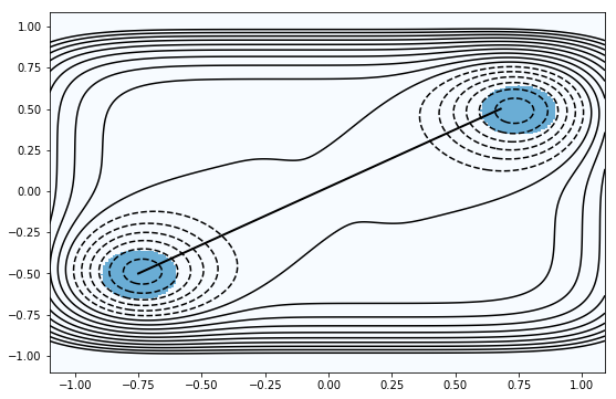
have a look at our potential, states and initial TP

plot = ToyPlot()
plot.contour_range = np.arange(-1.5, 1.0, .1)
plot.add_pes(pes_to_plot)
plot.add_states([stateA, stateB])

# passing the initial TP to bold and not to trajectories,
# because we want it to be....bold :)
fig = plot.plot(bold=[tra_to_2d(initAB)])

arcd setup

Create the underlying model to predict/fit the committors

The creation of the model naturally varies depending on the underlying model (e.g. Pytorch ANN) you chose.

# a collection of different pytorch ANN models can be found in arcd.pytorch.networks
# FFNet is a simple 4 layer feedforward network
# lets take 3 prediction networks
pnets = [arcd.pytorch.networks.FFNet(n_in=2 + n_harmonics,
                                     # using a single output we will predict only p_B and use a binomial loss
                                     # we could have also used n_out=n_states to use a multinomial loss and predict all states,
                                     # but this is only worthwhile if n_states > 2
                                     n_out=1
                                     )
         for _ in range(3)]
# and one calssifier to choose which prediction network is responsible for a certain point
cnet = arcd.pytorch.networks.FFNet(n_in=2 + n_harmonics,
                                   n_out=len(pnets)  # n_out for the classifier must be equal to len(pnets)
                                   )

# move model to GPU if CUDA is available
if torch.cuda.is_available():
    pnets = [pn.to('cuda') for pn in pnets]
    cnet = cnet.to('cuda')

# choose and initialize an optimizer to train the model
# Note that this should be done after moving the model where it should live (e.g. 'cuda')
# optimizer for prediction networks
poptimizer = torch.optim.Adam([{'params': pn.parameters()} for pn in pnets], lr=1e-3)
# optimizer for classifier
coptimizer = torch.optim.Adam(cnet.parameters(), lr=1e-3)

wrap the underlying model as arcd.RCmodel

• The subclass of arcd.RCModel depends on the underlying model(s). All arcd.RCModels for pytorch can e.g. be found in arcd.pytorch.rcmodel but are also imported to the topmodule arcd.pytorch, such that you can use them as arcd.pytorch.MODEL_CLASS.

• The arcd.RCModel and its subclasses is what you will usually be working with when using arcd. It is the expected input for the arcd.ops.RCModelSelector and arcd.ops.TrainingHook classes used for iterative training and also to all analysis methods that can be found in arcd.analysis. Normally there will be no need for you to access the underlying models, as all arcd.RCModels expose a consistent interface independent of the underlying model. This strict separation enables to easily add other underlying machine learning models to arcd by subclassing arcd.base.rcmodel.RCModel and simply adding the required functions without the need to reimplement the iterative training loop and decisions.

# we take an MultiDomain ExpectedEfficiencyPytorchRCModel,
# this RCmodel scales the learning rate by the expected efficiency factor (1 - n_TP_true / n_TP_expected)**2
model = arcd.pytorch.EEMDPytorchRCModel(pnets=pnets,
                                        cnet=cnet,
                                        poptimizer=poptimizer,
                                        coptimizer=coptimizer,
                                        gamma=-1,  # gamma is the exponent for the harmonic loss
                                        ee_params={'lr_0': 1e-3,  # lr = lr_0 * (1 - n_TP_true / n_TP_expected)**2
                                                   'lr_min': 1e-5,  # do not train if lr < lr_min
                                                   'epochs_per_train': 5,  # train for 5 epochs every time we train
                                                   'interval': 3,  # attempt to train after every 3rd MCStep
                                                   'window': 100,  # average expected efficiency factor over 100 MCSteps
                                                   },
                                        ctrain_params={'lr_0': 1e-3,  # lr = lr_0 * (1 - n_TP_true / n_TP_expected)**2
                                                       'lr_min': 1e-5,  # do not train if lr < lr_min
                                                       'epochs_per_train': 8,  # train for 8 epochs every time we train
                                                       'interval': 5,  # attempt to train after every 5rd MCStep
                                                       'window': 100,  # average expected efficiency factor over 100 MCSteps
                                                       },
                                        descriptor_transform=descriptor_transform,  # the function transforming snapshots to descriptors
                                        loss=None  # if loss=None it will choose either binomial or multinomial loss, depending on the number of outputs of the pnets,
                                        # but we could have also passed a custom loss function if we wanted to
                                        )

initialize an empty arcd.TrainSet

• The TrainSet is always the same for all RCModels, it stores the shooting points together with corresponding shot_results. It also has some useful methods to iterate over the training data.

• It needs to know about the states, such that it can extract the states reached from given OPS snapshots/trajectories and about the CV transforming molecular coordinates to training descriptors, such that it can calculate and store the training descriptors for each point.

trainset = arcd.TrainSet(states=[stateA, stateB], descriptor_transform=descriptor_transform)

create arcd.Trainhook

This is the object handling the interface between openpathsampling and the arcd.RCModel. It will train the model according to the models train_hook and train_decision() methods and save it after the TPS simulation (and every save_model_interval MCSteps). It will also try to load and reset the arcd.RCModel if continuing a TPS simulation from file.

trainhook = arcd.ops.TrainingHook(model=model,
                                  trainset=trainset,
                                  save_model_interval=200
                                  )

create acrd.ops.RCModelSelector

This is the object handling the selection of new shooting points according to the current arcd.RCModel prediction. It also calculates (part of) the acceptance factor for the TPS simulation. See openpathsampling.ShootingPointSelector for more on shooting point selectors in OPS.

selector = arcd.ops.RCModelSelector(model=model,  # always takes a RCModel
                                    # we can greatly speed up rejecting/accepting trial TPS by passing the list of states
                                    # this enables testing if a trial TP is even a TP and calculating the potentially costly
                                    # transformation from Cartesian to descriptor space only if neccessary
                                    # if we are lazy and know that the transformation is fast we can also explicitly pass None
                                    states=[stateA, stateB],
                                    # new shooting points are selected with p_sel(SP) ~ p_lorentz(model.z_sel(SP))
                                    # could also choose 'gaussian'
                                    distribution='lorentzian',
                                    # softness of the selection distribtion,
                                    # lower values result in a sharper concentration around the predicted transition state,
                                    # higher values result in a more uniform selection
                                    scale=1.0,
                                   )

setup openpathsampling TPS simulation and storage

This is basic openpathsampling stuff, please consult the openpathsampling examples for details on this section.

# velocity randomizer setup
beta = integ.beta
modifier = paths.RandomVelocities(beta=beta, engine=toy_eng)
# shooting strategy: TwoWayShooting
tw_strategy = paths.strategies.TwoWayShootingStrategy(modifier=modifier, selector=selector, engine=toy_eng, group='TwoWayShooting')
# transition network, tells us which transitions to sample
tps = paths.TPSNetwork.from_states_all_to_all([stateA, stateB])
# move scheme, tells us how to do the sampling
move_scheme = paths.MoveScheme(network=tps)
move_scheme.append(tw_strategy)
# this should always be the last added strategy for custom move_schemes, it sorts all previously appended strats when building the tree
move_scheme.append(paths.strategies.OrganizeByMoveGroupStrategy())
move_scheme.build_move_decision_tree()

# get initial conditions sample set from initial TP
initial_conditions = move_scheme.initial_conditions_from_trajectories([initAB])

No missing ensembles.
No extra ensembles.

# create a storage file
storage = paths.Storage('22dim_toy_MDpytorch.nc', 'w', template=template)

# create a PathSampling
sampler = paths.PathSampling(storage=storage,
                             sample_set=initial_conditions,
                             move_scheme=move_scheme
                             )

# THIS IS IMPORTANT
# make sure we save the descriptor_transform to storage,
# OPS will only save it if any other saved object contains a reference to it
# but we can esily save it ourselfes by doing
storage.save(descriptor_transform)

(store.attributes[PseudoAttribute] : 3 object(s),
 20,
 174916790489889098161946578561527709740)

arcd specific again: attach the TrainHook to the PathSampling such that it can train after every MCStep

sampler.attach_hook(trainhook)

# do 500 MCSteps of TPS
sampler.run(500)

Working on Monte Carlo cycle number 1000
Running for 20 minutes 48 seconds -  2.50 seconds per step
Estimated time remaining: 2 seconds
DONE! Completed 1000 Monte Carlo cycles.

Lets have a look at the training process

# train log_decision is a list of lists
# every entry contains [train, lr, epochs] as returned by model.train_decision()
print(model.log_train_decision[-1])

[False, 6.586498595766113e-06, 5]

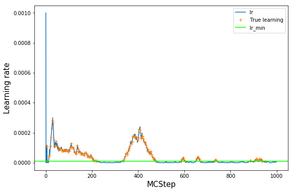
# lets have a look at the value of the learning rate over the course of training
# note however, that we did not train at every step, but just at every interval MCsteps
log_train = np.array(model.log_train_decision)
lr = log_train[:,1]
plt.plot(lr, label='lr')
# see where we really trained: everywhere where train=True
# set lr_true to NaN anywhere where we did not train to have a nice plot
lr_true = lr
lr_true[log_train[:,0] == False] = np.nan
plt.plot(lr_true, '+', label='True learning')
# lr_min as a guide to the eye
plt.axhline(model.ee_params['lr_min'], label='lr_min', color='lime')
plt.legend()
plt.xlabel('MCStep', size=15);
plt.ylabel('Learning rate', size=15);

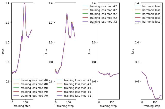
# the model losses at each step where it trained
# this will be epochs_per_training loss values per training
n_mod = len(model.pnets)
losses = np.array(model.log_train_loss)

min_val = np.min(losses)
max_val = np.max(losses)
fig, axs = plt.subplots(1, n_mod + 1)

for i, ax in enumerate(axs):
    label = 'training loss mod #{:d}'.format(i) if i < n_mod else 'harmonic loss'
    ax.plot(losses[:,:,i], label=label)
    ax.set_ylim(min_val, max_val)
    ax.set_ylabel('loss')
    ax.set_xlabel('training step')
    ax.legend()
fig.tight_layout()

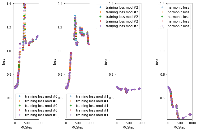
# resort such that we have a loss value per MCStep, NaN if we did not train at that step
train_loss = []
count = 0
for t in log_train[:, 0]:
    if t:
        train_loss.append(model.log_train_loss[count])
        count += 1
    else:
        train_loss.append([[np.nan for i in range(len(model.pnets)+1)] for _ in range(model.ee_params['epochs_per_train'])])


losses = np.array(train_loss)
min_val = np.min(model.log_train_loss)
max_val = np.max(model.log_train_loss)
fig, axs = plt.subplots(1, n_mod + 1)

for i, ax in enumerate(axs):
    label = 'training loss mod #{:d}'.format(i) if i < n_mod else 'harmonic loss'
    ax.plot(losses[:,:,i], '+', label=label)
    ax.set_ylim(min_val, max_val)
    ax.set_ylabel('loss')
    ax.set_xlabel('MCStep')
    ax.legend()
fig.tight_layout()

# get the number of accepts from OPS storage
accepts = []
for step in storage.steps:
    if step.change.canonical.accepted:
        accepts.append(1.)
    else:
        accepts.append(0.)

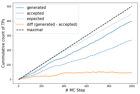
# plot efficiency, expected efficiency and accepts
# Note: this will only work for models with n_out=1, due to the way we calculate p(TP|x)

p_ex = np.array(model.expected_p)

l, = plt.plot(np.cumsum(trainset.transitions), label='generated');
plt.plot(np.cumsum(accepts), c=l.get_color(), ls='--', label='accepted');
plt.plot(np.cumsum(2*p_ex*(1 - p_ex)),c=l.get_color(), ls=':', label='expected');
plt.plot(np.cumsum(2*p_ex*(1 - p_ex))- np.cumsum(trainset.transitions), label='diff (generated - accepted)')
plt.plot(np.linspace(0., len(trainset)/2., len(trainset)), c='k', ls='--', label='maximal', lw=2)
plt.legend(fontsize=15);
plt.ylabel('Cummulative count of TPs', size=15)
plt.xlabel('# MC Step', size=15);

look at what the model learned

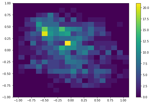
# have a look at the distribution of SPs in the x/y plane
# should show us that the model concentrates the SPs around the transition state in x/y
# Note that this is not really helpful in a molecular setting, as we ussually do not know the projection
# in which the high dimensional descriptor input space reduces to easy relations
# However, for our toy example it can be quite instructive to look at. 

x = np.zeros((len(storage.steps)-1,))
y = np.zeros((len(storage.steps)-1,))
for i, step in enumerate(storage.steps[1:]):
    coords = step.change.canonical.details.shooting_snapshot.coordinates[0]
    x[i] = coords[0]
    y[i] = coords[1]

# the whole history
plt.hist2d(x, y, range=[(-1.1, 1.1),(-1., 1.)], bins=20)
plt.colorbar();

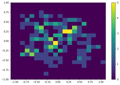
# the first 200 steps
plt.hist2d(x[:200], y[:200], range=[(-1.1, 1.1),(-1., 1.)], bins=20)
plt.colorbar();

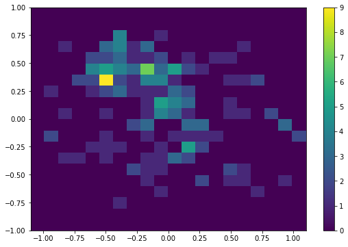
# the last 200 steps
# hopefully there will be a difference... :0
plt.hist2d(x[-200:], y[-200:], range=[(-1.1, 1.1),(-1., 1.)], bins=20)
plt.colorbar();

# we can also have a look at the models prediction in x/y
# we take the surface where all oscillators are 0
x = np.linspace(-1.2, 1.2, 240)
y = np.linspace(-1., 1., 200)

# matrix for the classifier weighted prediction
pred = np.zeros((len(y), len(x), 2))
# matrix for the classifier prediction
pred_c = np.zeros((len(y), len(x), len(model.pnets)))
# list of matrixes of single model predictions
pred_single = [np.zeros((len(y), len(x), 2)) for _ in range(len(model.pnets))]

random_osci_values = False
if random_osci_values:
    # draw a x at random from Boltzmann, compatible with omega of the oscillator
    # takes quite a bit longer...    
    for i, xv in enumerate(x):
        for j, yv in enumerate(y):
            coord = np.array([[xv, yv] + [np.random.normal(scale=np.sqrt(1./(10.*pes_list[-1].omega[i+2]**2))) for i in range(n_harmonics)]])
        
            p, p_single = model(coord, use_transform=False, domain_predictions=True)
            pred[j,i, 1] = p[0]
            pred[j,i,0] = 1 - p[0]
            for k, p_s in enumerate(p_single):
                pred_single[k][j,i,1] = p_s[0]
                pred_single[k][j,i,0] = 1 - p_s[0]
        
            pred_c[j,i] = model.classify(coord, use_transform=False)
else:
    # we take the surface where all oscillators are 0
    oscis = [0.0 for _ in range(n_harmonics)]
    # do one prediction for one big vector and unwrap it afterwards
    # this is much faster than looping over the single coordinate points as we can make use of the GPU/CPU vector operations...!
    coord = np.array([[xv, yv]  + oscis for yv in y for xv in x])
    p, p_single = model(coord, use_transform=False, domain_predictions=True)
    p = p.reshape((len(y), len(x)))
    pred = np.stack([1. - p, p], axis=-1)
    for k, p_s in enumerate(p_single):
        pred_single[k][:, :, 1] = p_s.reshape((len(y), len(x)))
        pred_single[k][:, :, 0] = 1 - p_s.reshape((len(y), len(x)))
    
    pred_c = model.classify(coord, use_transform=False)
    pred_c = pred_c.reshape((len(y), len(x), len(pnets)))

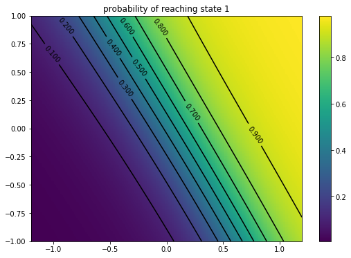
# plot committement probability towards state B
s_num = 1

fig, ax = plt.subplots(1)
im = ax.imshow(pred[...,s_num], origin='lower', extent=(x[0], x[-1], y[0], y[-1]))
levels = np.arange(0., 1., 0.1)
X, Y = np.meshgrid(x, y)
CS = ax.contour(X, Y, pred[..., s_num], levels, colors='k')
ax.clabel(CS, inline=1, fontsize=10, )

ax.set_title('probability of reaching state {:d}'.format(s_num))
fig.colorbar(im);

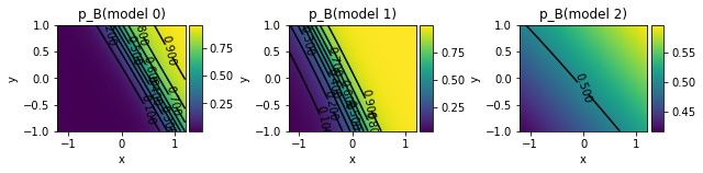
# plot single model predictions
from mpl_toolkits.axes_grid1 import make_axes_locatable
fig, axs = plt.subplots(1, len(model.pnets))
X, Y = np.meshgrid(x, y)

for mod_num, p in enumerate([pred_single[i][:,:,1] for i in range(len(model.pnets))]):
    ax = axs[mod_num]
    ax.set_xlabel('x')
    ax.set_ylabel('y')
    im = ax.imshow(p, origin='lower', extent=(x[0], x[-1], y[0], y[-1]))
    
    CS = ax.contour(X, Y, p, levels, colors='k')
    ax.clabel(CS, inline=1, fontsize=10, )
    ax.set_title('p_B(model {:d})'.format(mod_num))
    divider = make_axes_locatable(ax)
    cax = divider.append_axes("right", size="10%", pad=0.05)
    #color_ax = fig.add_axes()
    fig.colorbar(im, cax=cax, orientation='vertical')
fig.tight_layout()

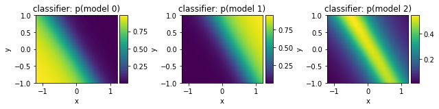
# plot classifier model weights
from mpl_toolkits.axes_grid1 import make_axes_locatable
fig, axs = plt.subplots(1, len(model.pnets))

for mod_num, p in enumerate([pred_c[:,:,i] for i in range(len(model.pnets))]):
    ax = axs[mod_num]
    ax.set_xlabel('x')
    ax.set_ylabel('y')
    im = ax.imshow(p, origin='lower', extent=(x[0], x[-1], y[0], y[-1]))
    ax.set_title('classifier: p(model {:d})'.format(mod_num))
    divider = make_axes_locatable(ax)
    cax = divider.append_axes("right", size="10%", pad=0.05)
    #color_ax = fig.add_axes()
    fig.colorbar(im, cax=cax, orientation='vertical')
fig.tight_layout()

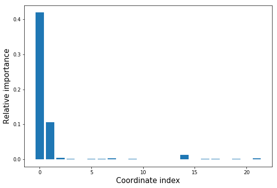
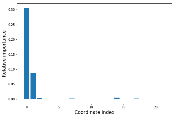
HIPR - relative input importance analysis

# perform a HIPR analysis of the model over the trainset
hipr = arcd.analysis.HIPRanalysis(model,
                                  trainset,
                                  n_redraw=5,  # setting n_redraw=5 will redraw random values 5 times for every descriptor dimension for every point 
                                  )

hipr_losses = hipr.do_hipr()  # the n_redraw given to do_hipr() directly takes precedence over the one given at init time

loss_diffs = hipr_losses[:-1] - hipr_losses[-1]  # hipr_losses[-1] is the reference loss over the unaltered trainset

plt.bar(np.arange(len(loss_diffs)), loss_diffs)
plt.xlabel('Coordinate index', size=15)
plt.ylabel('Relative importance', size=15);

hipr_plus_losses = hipr.do_hipr_plus()

loss_diffs = hipr_plus_losses[:-1] - hipr_plus_losses[-1]  # hipr_losses[-1] is the reference loss over the unaltered trainset

plt.bar(np.arange(len(loss_diffs)), loss_diffs)
plt.xlabel('Coordinate index', size=15)
plt.ylabel('Relative importance', size=15);

# sync and close the OPS storage
# not strictly neccessary but a good habit to make sure everything you expect is in there
storage.sync_all()
storage.close()